December 4th, 2024
T-Test In-Depth Guide
By Connor Martin · 6 min read

You want to evaluate if there’s any significant difference between a mean you’ve hypothesized and the actual mean presented in a data sample.
Enter the t-test – a statistical test you can use to find out if that mean difference exists and how large it is. Best used when you have 30 sample observations or less (though it can be used for larger datasets if they’re normalized), the t-test is among the handiest of statistical tools.
Key Takeaways
- T-tests identify significant differences between means: Use t-tests to determine whether the mean of one or two datasets differs significantly from a hypothesized mean or another group’s mean, especially when working with smaller, normally distributed data samples.
- Different t-test types suit specific scenarios: One-sample, independent, and paired t-tests address distinct comparison needs, from single dataset analysis to evaluate differences between two independent or paired groups.
- Key assumptions and alternatives matter: T-tests require normality and homogeneity of variance; when these assumptions don’t hold, alternatives like ANOVA or Mann-Whitney U tests may be better suited.
What Is a T-Test?
As touched on above, a t-test allows you to figure out the differences between the means of up to two datasets. That means that no more than two groups are allowed. The variable used in this test must be numeric, which limits the types of datasets you can use. Examples of appropriate datasets include gross profit, height, or age.
Understanding the Basics of T-Tests
The tricky part about t-tests is that there are several versions, each with particular use cases. So, let’s look at why you’d use a t-test first, and the purposes each version serves.
When and Why to Use a T-Test
Use a t-test when you have a small (likely random) sample containing up to 30 observations. These observations, which can be pulled from a larger statistical population, form a dataset. Your goal with the test is to compare the mean from your sample data with another value. That gives you the t-value or t-score, representing the variation between your sample sets.
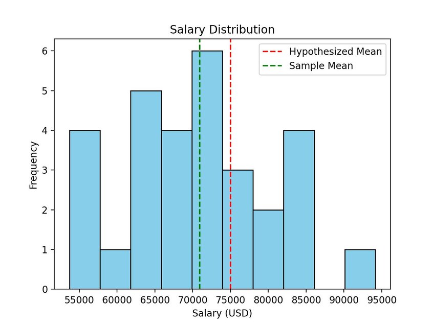
For instance, let’s say that you want to figure out the average salary for a group of people within a specific profession. A t-test works well here. You’d pull salary data randomly from up to 30 people and then apply the test to check what you think the mean salary is versus what it actually is.

Types of T-Tests
Though they sound simple on the surface, the type of t-test you use determines how successful your statistical analysis will be. Specifically, each t-test offers variations in the number of samples and variables you can use and the degrees of freedom available to you. These “degrees” are the number of independent variables that you can reasonably estimate using the t-test before putting constraints in place or moving on to another form of statistical test.
Understanding these different test types is crucial, and there are three that you need to know about.
One-Sample T-Test
Use a one-sample t-test when a single variable offers a continuous measurement. The salary example we used earlier would work here. You’re looking to see if the sample set’s mean equals the value you hypothesized before the test. Your degrees of freedom with this type of t-test are the number of observations in your dataset minus one. Use sample standard deviation for this type of t-test, as it’s unlikely you’ll have another population standard deviation available.
Independent (Two-Sample) T-Test
An independent t-test changes your degrees of freedom to the sum of the observations in your dataset minus two. This is also one of the two t-tests you can use if you have a pair of variables to define your groups. These variables can either offer a continuous measurement or be categorical or nominal.
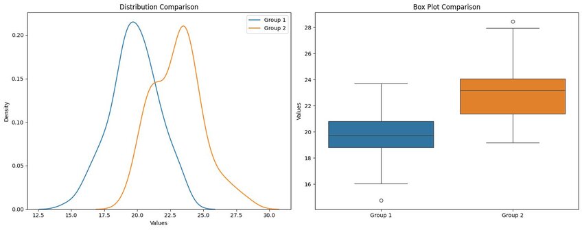
In our salary example, you can use an independent t-test to determine if the mean salaries between two random groups of people from the same industry are the same. This version of the test's purpose is to decide whether or not the mean values for two population groups are equal. Again, the sample standard deviation for each group is the norm for these tests.
Paired (Dependent) T-Test
Another t-test that requires two variables is the paired samples t-test, which shows whether the difference in the means between two sample groups is zero. In our salary example, you’ll get a zero difference if the mean salaries between your groups are the same. Your degrees of freedom with this test are the number of paired observations in your sample minus one.
So, you’re checking to confirm that there’s no difference in the results between the two groups. Again, you’ll use sample standard deviation in this test. However, you’ll use the differences between your paired samples in this case.
Key Assumptions for Conducting a T-Test
Before running a t-test, there are several assumptions about your sample(s) that you should feel comfortable making. If none of these assumptions are true in your case, it may be best to try an alternative test that allows you to work with data outside the constraints of a t-test.
Normality Assumption
Wild variations in your data objects will wreak havoc on a t-test because you have a distorted median. So, you have to be able to assume that you have normally distributed data, which means checking that your sample matches the Gaussian distribution bell curve.
Homogeneity of Variance
Homogeneity of variance refers to the variability of the data within your sample. For a t-test, you want that variability to be “similar,” which means there are no wild swings in data values.
Step-by-Step Guide to Performing a T-Test
Once you’ve chosen the appropriate t-test for your datasets, variables, and hypothesis, you’re ready to actually run the test. The steps tend to be the same regardless of the type of test you choose.
Step 1 - Data Collection and Preparation
The simplest of the steps involves gathering your data for the t-test. Coming back to our salary example, this could involve pulling up to 30 salaries randomly from a larger dataset to get your sample.
Step 2 - Setting Up the Hypotheses
Your hypotheses steer your entire analysis, so you need to have them in place before you run your t-test. You’ll likely start with a null hypothesis stating that there will likely be no significant difference between your estimation of the mean values within your datasets and what they actually end up being. Your alternative hypothesis essentially says the opposite – that there is a significant difference, and your t-test will demonstrate it.
Step 3 - Calculating the T-Statistic and P-Value
Here’s where we start digging into some notation. Again, we’ll use our salary example with a null and alternative hypothesis. The null hypothesis is that there is zero difference between our estimated mean and our tested mean, with the alternative representing any difference between them. So, we’ll have the following:
H0: µ = 0
Ha: µ ≠ 0
Where “H0” is our null hypothesis and “Ha” is our alternative.
With that, we can use the following formula to determine our t-statistic:
t = (x̅-μ) / (s/√n)
Here, “x̅” is our sample mean, with “μ” being our hypothesized mean. “s” and “n” are much more straightforward: the former is our sample standard deviation, and the latter is our sample size.
The formula gives us a value for “t.”
However, finding the p-value is a far trickier task. To do it by hand, we’d need to use a t-distribution table that accounts for the degrees of freedom relevant to our t-test. It’s far easier to use an online calculator or statistical software such as Julius AI to find this value.
Step 4 - Interpreting Results
Once you’ve found your p-value, you’ll also be able to see the two alpha levels with which they correspond. Also dubbed “significance levels,” the alpha levels tell you the probability that you will have to reject your null hypothesis. Check your p-value against your chosen alpha level. If the p-value is less than your alpha level, then your null hypothesis is accurate.
Practical Examples of T-Tests in Use
We’ve already touched on a basic example of using a t-test to determine the mean salary within a specific industry. Here are a few more situations when this type of statistical test might prove helpful.
Example: Comparing Two Means in Medical Studies
Let’s say you want to test the effect of a new medication on patient blood pressure. You’d have test subjects with high blood pressure placed into two sample groups – a placebo group and a group taking your new medication.
After running your study for however long is required, you’d take the results and place them into a two-sample t-test. This t-test will reveal whether there’s a significant – and, in this case, expected – variance between the mean values you pull from your placebo and medication test groups.
Example: Business Applications of T-Tests
Suppose you run a business and want to see if the mean salary you offer for a specific role aligns with the mean salary in the wider industry. The t-test is your friend here – it allows you to check your mean salary against a wider mean so you can tweak your offer accordingly.
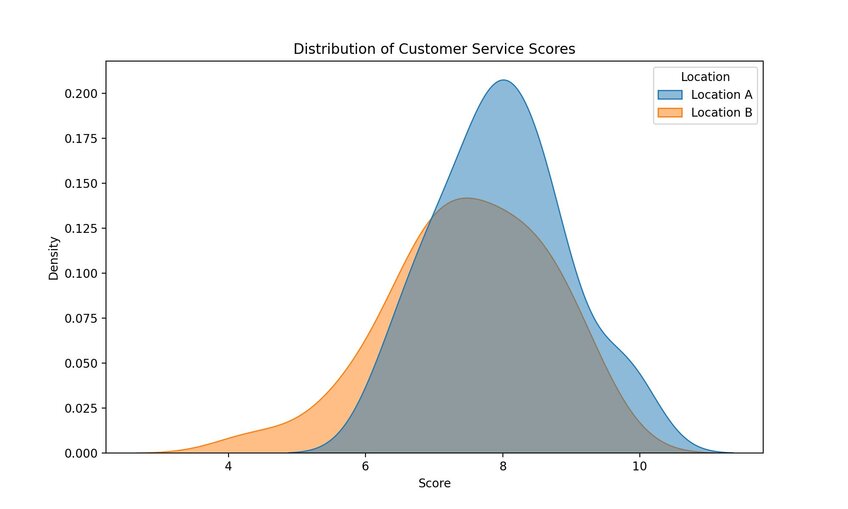
Beyond that, you could use t-tests for a host of other business purposes. Comparing the quality of customer service between locations based on scores given by your clients is a good example, as is measuring employee performance. In fact, any number-based metrics that you have can be subjected to t-tests.

T-Test Formulas and Calculation
This being the field of statistics, there are, of course, formulas that we need to cover if you’re going to run a t-test manually. Each of these formulas gives you a t-statistic from which you can determine the p-value used to analyze your results.
The following variables apply to each formula:
X̅ = Sample Mean
μ = Hypothesized Mean
s = Sample Standard Deviation
n = Sample Size
In some of the formulas below, you’ll see a number next to one of these letters, such as “n2.” This number denotes the dataset from which the number comes. So, “n2” means the sample size from your second dataset.
Formula for a One-Sample T-Test
The one-sample t-test formula is the same one that we used in the steps outlined earlier:
t = (x̅-μ) / (s/√n)
Formula for an Independent T-Test
Things get a little more complicated with an independent t-test because you’re working with two variables and datasets.
t = x̅1 – x̅2 / Sp Ö1/n1 + 1/n2
For this equation, Sp is the pooled standard variation.
Formula for a Paired T-Test
The paired t-test is a little more complicated than the previous two formulas because you’re throwing differences into the mix. So, we have to add the following symbols:
D = Differences between Your Two Paired Samples
di = The ith Observation within D
d̅ = Sample Mean of the Differences
σ^ = Sample Standard Deviation of the Differences
All other letters and symbols used have the same meaning as defined above. For a paired t-test, you start by calculating your sample mean with this formula:
d̅ = d1 + d2 + … + dn / n
That gives you “d̅,” which you then plug into the following equation to derive your sample standard deviation:
σ^ = Ö(d1 – d̅)2 + (d2 – d̅)2 + …. + (dn – d̅)2 / n – 1
Finally, you can derive your t-statistic:
t = d̅ - 0 / σ^ / Ön
T-Test Interpretation and Common Mistakes
Just looking at the complexity of some of these formulas, you can see that it’s pretty easy to make mistakes with t-tests if you’re doing them manually. Look out for these mistakes and misinterpretations – all can lead to inaccurate results.
What Does the P-Value Mean?
P-value stands for “probability value.” It tells you how likely it is that your null hypothesis is correct based on the t-test conducted on your sample data. The smaller your p-value is, the more likely that your null hypothesis is correct.
Common Misinterpretation and Pitfalls
Perhaps the most common misinterpretation of a t-test is that it’s only useful for smaller datasets. That’s true in most cases – you’ll get the best out of these tests with a sample containing less than 30 objects.
However, t-tests are also useable on larger datasets. The key is that your sample data has to be somewhat normally distributed, which becomes harder to achieve when you’re working from a larger sample.
As for pitfalls, the normalized distribution factor comes into play again. If your data varies wildly to the point where it doesn’t fit the Gaussian distribution bell curve model, it’s a bad idea to run a t-test.
Alternatives to T-Tests
A good t-test relies on you being able to make the assumptions we mentioned earlier. If that isn’t possible, you need an alternative.
ANOVA (Analysis of Variance)
ANOVA is an appropriate test when you have more than two data samples to work with. T-tests can’t handle more than two groups, but ANOVA tests can. So, switch to this type of test when you’re working with multiple samples.
Mann-Whitney U Test
What can you use when you want to run an independent sample t-test, but your data isn’t normalized? A Mann-Whitney U Test is the answer. It provides the same types of answers as a t-test but can handle un-normalized datasets.
Discover How Julius Can Make T-Test and Other Statistical Analysis Simple
Why struggle with manually porting numbers into complex formulas when you can use a tool to run your t-tests in seconds? That’s what Julius AI offers. It’s your go-to tool for chatting with files and datasets, allowing you to pull whatever insights you need from the data you enter. That includes running t-tests. Just ask Julius AI to find the mean value of your sample, and you can test your null hypothesis in seconds.
Does that sound good? Try Julius AI today – and make t-tests a breeze from now on.
Frequently Asked Questions (FAQs)
What does a t-test tell you?
A t-test evaluates whether there is a statistically significant difference between the means of two datasets or between a sample mean and a hypothesized mean. It quantifies the size of this difference while accounting for variability within the data, helping you determine if the observed differences are due to chance.
What does a positive t-test mean?
A positive t-test result means the sample mean is higher than the hypothesized mean or the mean of the second group, depending on the type of t-test used. However, the sign of the t-value doesn’t affect the interpretation of significance, which depends on the p-value and chosen alpha level.
When to use ANOVA vs. t-test?
Use a t-test when comparing the means of two groups or one sample mean against a hypothesized value. ANOVA is better suited for comparing means across three or more groups, as it can handle multiple datasets while maintaining statistical accuracy.
When to use the t-test and z-test?
A t-test is ideal for small sample sizes (typically less than 30) or when the population standard deviation is unknown. A z-test is used for larger samples (typically over 30) when the population standard deviation is known, as it assumes the data follows a normal distribution.
What is the t-test between two groups?
The t-test between two groups, also known as an independent t-test, compares the means of two separate datasets to determine if the difference is statistically significant. It’s commonly used in scenarios like testing differences in performance, salaries, or treatment effects across two independent groups.
