March 5th, 2024
Your Guide to Understanding Path Analysis in Statistics
By Alex Kuo · 8 min read
The world is full of constantly changing and seemingly random variables: raw data that’s loud, disorganized, and chaotic. As a statistician, your job is to organize this chaos into a manageable and readable form that draws together patterns and determines trends.
This is often done by comparing data sets with each other.
Structural equation modeling (SEM) is the statistical approach that allows analysts to draw connections between these observed variables and any underlying latent variable models to extrapolate how one set of variables predicts another. Of the various regression models that can be used to get this done, there’s path analysis.
What does it do and why does it matter? Let this article be your guide.
What Is Path Analysis?
Quite simply, path analysis is a method of analyzing the direct and indirect effects of differing variables, over several causal branches, on the outcome of an event.
It was developed by U.S. geneticist Sewall Wright for use in agriculture and the environment. Though it was slow to catch on, today it’s widely used across several fields (including biology, economics, and social sciences) to determine the role that variables in a system have on a particular outcome.
Statistics typically rely on two variables:
- Independent variables (IVs) – The variable that can be changed to observe its effect on another variable.
- Dependent variables (DVs) – The variable being observed by the method, underpinning the process.
This is a perfectly fine approach for simple models with easily definable causation. One or two IVs directly affect the DV without interaction or non-recursion. But what if there’s a middle step between the two groups? What happens when different IVs affect each other? Can they still be independent?
That’s where path analysis in statistics comes in.
Doing away with IVs and DVs, this method instead rebrands all variables as either:
- Exogenous – A variable that acts on one or more other variables without being impacted in turn (excluding error terms of course)
- Endogenous – These have at least one exogenous variable acting on them
This classification allows for more complex models (or “paths”) to be devised and can compare data in even more complex scenarios. These are laid out in a path diagram, and an equation is then derived from the different variables. These themselves can be grouped into one of two categories:
1. Interdependent model – Your standard multiple regression path model. The exogenous variables aren’t correlated with each other and affect one or more endogenous variables.
2. Mediated (indirect) model – Exogenous variables in this path model act upon intermediate endogenous variables, thus having some effect on the final endogenous cause.
Errors, be they through data imprecision or human mistakes, are also factored into the mix with path analysis, through the addition of “disturbances.” Even though errors can be reduced with the help of tools like Julius AI, life is still complex. These terms are added to every endogenous variable by default and can be drawn or omitted from the pathing diagram.

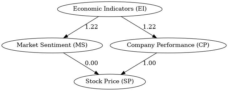
Example path analysis that illustrates how Economic Indicators directly influence Market Sentiment and Company Performance, which in turn directly affect Stock Price. The coefficients on the edges quantify the strength of these relationships. Created in seconds with Julius AI
Why Is It Important?
The primary use of path analysis is comparison. If you want to find out why bad weather affects low attendance at a school, you’ll need to include one or more variable sets (transport, reluctance, distance, danger) to see which affects the outcome and which matters the most.
Path analysis’s structure also allows it to handle more complex models than other multiple regression models, allowing for more in-depth comparison. Even better, different models can be compared with each other to determine the best fit for data. This results in clearer hypotheses and more plausible pathways. With the aid of AI tools like Julius, variables, and models can be produced in a fraction of the time.
That said, path analysis isn’t without its limitations. In addition to developing path analysis, Sewall Wright also coined the famous term: “Correlation doesn’t equal causality.” Path analysis was once called “causal modeling” with the erroneous assumption that one could derive causality from the model. Sadly, that’s not the case.
The models can only work with the variables they have and longitudinal studies and the like have to pick up the slack.
What’s more, path analysis completely breaks down with feedback loops, or recursive, modeling. In life, everything is interconnected, but in statistics, such interdependency works against the model in the long run and does more harm than good.
Finally, path analysis needs some help in determining the flow of causality. The statistician must have prior knowledge of possible causes to devise a working model. It’s good, but not that good.
How to Conduct Path Analysis
Any effective path analysis approach follows the same rough outline:
1. The model is conceptualized – Create the path diagram, including all the exogenous and endogenous variables, being sure to define their relationship to each other. The direction must be decided and the steps chosen along the way.
2. Data is gathered – Every good model needs data. Once your variables have been identified, you’ll need to gather enough substantial data for it to be viable. This can be conducted online or through focus groups.
3. Software is chosen – You’ll need the right tools for the job. SPSS and STATA are good tools, but machine learning options like Julius AI can be more flexible and faster when it comes to remodeling, input, and calculation.
4. Statistical analysis – Estimate the model using the derived equation and methods like maximum likelihood. Be sure to obtain both standardized and unstandardized path coefficients, correlation coefficients, measurement errors, outliers, and any other important details.
5. Comparison and refinement – With your data on hand, it’s time to demonstrate the actual correlation between variables through the correlation matrix. The model can be tweaked and new data added to refine the outcome variables. Compare both input and output path diagrams to see whether your initial causal hypothesis is supported. Fine-tune if necessary.
How You Can Use Path Analysis
Path analysis may have begun life in the agricultural sector, but its uses stretch far and wide into a myriad of different real-life applications. It’s all about comparison and relationships. Here are just a few examples:
- Marketing – Researchers can determine what factors affect consumers’ purchasing decisions and take more informed actions based on this behavior.
- Healthcare – You can investigate the role that certain factors play in the effectiveness of healthcare treatments (e.g. genetics, age, BMI).
- Social Studies – Overarching social behaviors and conventions can be compared against individual actions and choices to determine their impact.
- Business – The financial world uses path analysis to determine the various factors that are positively or negatively impacting their businesses and profits and adjust to improve their business outcomes.

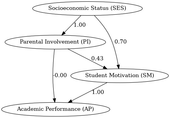
Example path analysis that illustrates how Socioeconomic Status directly influences Parental Involvement and Student Motivation, which in turn directly affects Academic Performance. The coefficients on the edges quantify the strength of these relationships. Created in seconds with Julius AI
Use Julius AI for Path Analysis and Other Statistical Processes
Effective path analysis requires the quick processing of large amounts of data. You’ll need to compare models and swap out variables quite frequently on the way to success. You need a tool that can respond just as quickly. Julius AI offers you answers to your data questions, sleek visualizations, automated data prep, instant exports, and much more. It’s more than a tool: it’s a partner in your research.
Frequently Asked Questions (FAQs)
How to interpret path analysis results?
Path analysis results are interpreted by examining the path coefficients, which indicate the strength and direction of the relationships between variables. Positive coefficients suggest a direct relationship, while negative ones indicate an inverse relationship. Comparing the coefficients helps identify the most influential variables in the model.
What is the difference between regression and path analysis?
While regression focuses on the relationship between independent and dependent variables, path analysis extends this by analyzing both direct and indirect effects across multiple causal pathways. Path analysis also allows for the inclusion of intermediate (mediating) variables and distinguishes between exogenous and endogenous variables.
What statistical tool is used for path analysis?
Common statistical tools for path analysis include software like SPSS, STATA, and Amos. For more advanced and flexible modeling, machine learning tools such as Julius AI can streamline the process with faster computations and user-friendly visualizations.
What is an example of a path analysis?
An example of path analysis might explore how socioeconomic status influences parental involvement and student motivation, which in turn affects academic performance. By analyzing the coefficients, researchers can determine which factors are most impactful and how they interconnect.
